Diffusion Models

Take a clean image and add a little noise. Add a little more. Keep going for a few hundred steps and you end up with static, an image indistinguishable from random noise. That destruction is easy and needs no learning at all; it is just repeated addition of noise. The insight behind diffusion models is that if a network could learn to undo one step of that process, to look at a slightly noisy image and predict the noise that was added, then you could run the whole thing backward. Start from pure noise, subtract the predicted noise step by step, and a coherent image emerges that was never in the training set.

The idea

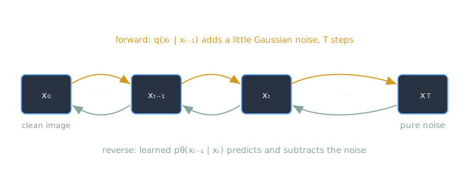
A diffusion model, made practical by Ho and colleagues in 2020 (the DDPM paper), defines a fixed forward process that gradually corrupts data into noise over $T$ steps, then learns the reverse. A network is trained to predict the noise present in a partially corrupted image. To generate, sample pure noise and apply the learned denoiser repeatedly, walking the chain backward from noise to a clean sample. The name comes from modeling a diffusion process in thermodynamics.

The Forward Process: Scheduled Destruction

The forward process is a fixed recipe, not something the model learns. Starting from a clean image $x_0$, each step produces a slightly noisier version by mixing in a bit of Gaussian noise:

$q(x_t\mid x_{t-1})=\mathcal{N}\left(x_{t-1}\sqrt{1-{\beta }_t},{\beta }_{t}I\right)$

Here ${\beta }_t$ is a small variance that controls how much noise enters at step $t$, set by a schedule chosen ahead of time. Each step nudges the image toward randomness and scales down what remains of the signal. Repeat for $T$ steps and $x_T$ is essentially a sample of pure noise, all trace of the original image gone. Because every step just adds known Gaussian noise, there is no learning here. The forward process exists only to manufacture training pairs: a noisy image and the exact noise that was put into it.

The Reverse Process: Learned Denoising

Undoing the noise is where the network comes in. The model learns the reverse transition $p_{\theta }(x_{t-1}\mid x_t)$: given a noisy image at step $t$, recover a cleaner image at step $t-1$. In practice the network is trained to predict the noise that was added at that step, which is a plain regression target trained with gradient-descent. The architecture that carries this is typically a U-Net, an encoder-decoder with skip connections (the same shape used in image segmentation), which takes a noisy image and the step index and outputs a noise estimate the same size as the image.

The training loop is a direct consequence of the setup. Pick a training image, pick a random step $t$, run the forward process to noise it up to $x_t$ while keeping the noise you added, and ask the network to predict that noise from $x_t$. The loss is the error between the predicted noise and the actual noise. Because the forward process hands you a perfect target for free, the whole thing trains without labels, a form of unsupervised-learning on the data itself.

Generation: Walking the Chain Backward

Sampling is the reverse process run end to end.

1. Sample $x_T$ from a standard Gaussian $\mathcal{N}(0,I)$, pure noise.
2. Feed the current image and step to the network to predict the noise in it.
3. Use that predicted noise to take one small step toward a cleaner image, $x_{t-1}$.
4. Repeat, stepping $t$ down until you reach $x_0$, a finished image.

Nothing about $x_T$ came from the training set, so the output is genuinely new. This is what puts diffusion in the same family as the variational autoencoder and the GAN: all three sample new data by pushing random noise through a learned map. The routes differ. A VAE decodes a single draw from an organized latent prior, a GAN generates in one forward pass judged by an adversary, and a diffusion model reaches the image through many small denoising steps. That iterative refinement is slower to sample but tends to train stably and produce high-fidelity, diverse output, sidestepping the mode collapse that plagues GANs.

Example

Stable Diffusion generates images from text prompts and runs on consumer hardware with slightly fewer than $10^9$ parameters. It adds two tricks to the basic recipe. It runs the diffusion process in a compressed latent space rather than on raw pixels, so an autoencoder shrinks the image first and expands the result at the end, which is far cheaper. And it conditions the denoising U-Net on the text prompt through cross-attention, so the noise the network predicts depends on the words. Prompt it with “a photograph of an astronaut riding a horse” and the backward walk from noise lands on exactly that, an image that has never existed.

Related Notes

• artificial-neural-networks provide the U-Net denoiser at the core of the reverse process
• normal-distribution defines both the noise added forward and the starting point for generation
• loss-functions and gradient-descent train the network to predict noise
• unsupervised-learning because the forward process supplies its own training targets, no labels needed
• autoencoders and generative-adversarial-networks are the sibling generative models; diffusion reaches an image through many denoising steps rather than a single decode or an adversarial pass
• features-and-representations on why running diffusion in a compressed latent space is cheaper
• ai-vs-ml-vs-dl for where generative deep learning sits in the bigger picture

Sources

• https://arxiv.org/abs/2006.11239 (Ho, Jain & Abbeel, 2020, “Denoising Diffusion Probabilistic Models”: the forward noising process, the noise-prediction training objective, and the reverse sampling procedure)
• https://en.wikipedia.org/wiki/Diffusion_model (forward and reverse Markov chains, the variance schedule, U-Net denoiser, connection to thermodynamic diffusion)
• https://arxiv.org/abs/1505.04597 (Ronneberger, Fischer & Brox, 2015, “U-Net”: the encoder-decoder-with-skip-connections architecture used as the denoiser)
• https://www.deeplearningbook.org/contents/generative_models.html (Goodfellow, Bengio, Courville, Deep Learning, ch. 20: deep generative models, the family diffusion belongs to)
• Course framing: CSCE 479/879 (Stephen Scott, UNL), “Autoencoders, GANs, and Diffusion Models” lecture slides