Backpropagation

A single unit is easy to train because you can see how each weight touches the output. A deep network is not, because a weight in an early layer influences the loss only through a long chain of later units. To improve that weight with gradient-descent you need its partial derivative of the loss, and computing all of those derivatives by hand, one per weight, would be hopeless for a network with millions of them. Backpropagation is the bookkeeping that makes it tractable: it computes every gradient in a single organized sweep backward through the network, reusing work at each step.

The idea

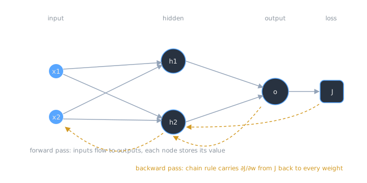
Backpropagation computes the gradient of the loss $J$ with respect to every weight by applying the chain rule from the output backward to the inputs. Represent the network as a computation graph of simple operations. In one forward pass each node records its value; in one backward pass each node multiplies the gradient arriving from downstream by its own local derivative and passes the product upstream. Because each intermediate result is computed once and reused, the whole gradient costs about as much as the forward pass.

The Computation Graph

Write the network as a computation graph, the same structure a framework like TensorFlow builds internally. Each node is a primitive operation (a multiply, an add, an exponential, a division), edges carry values, and the final node is the loss $J$. A complicated function $f(\mathbf{w},\mathbf{x})$ becomes a chain of tiny functions, and the key point is that every primitive has a local derivative you already know. Multiplication, addition, and the activation functions all have simple, closed-form derivatives.

The forward pass just evaluates the graph left to right on a given input, and each node stores the value it produced. Those stored values are exactly what the backward pass will need.

The Backward Pass

Now walk the graph in reverse. Seed the output with $\frac{\partial J}{\partial J}=1$. At every node, take the gradient flowing in from its downstream neighbor and multiply by the node’s own local derivative. That product is the gradient with respect to the node’s inputs, which you then send further upstream. This is nothing more than the chain rule, $\frac{\partial J}{\partial a}=\frac{\partial J}{\partial b}\frac{\partial b}{\partial a}$, applied one edge at a time.

When a value feeds more than one downstream node, the multivariate chain rule says to sum the contributions along every path from $J$ back to that value. Adding up the paths is the only wrinkle, and it falls out of the same mechanical rule.

Why It Is Efficient

The reason backpropagation wins is reuse. The gradient at an early layer is built from gradients already computed at later layers, so nothing downstream is recalculated. Once you have $\frac{\partial J}{\partial b}$ for some node, computing $\frac{\partial J}{\partial a}$ for the node feeding it is a single local multiplication, and it does not matter whether that node is near the output or deep inside the network. You can run the process indefinitely backward.

Formally, backpropagation is a special case of reverse-mode automatic differentiation. This modularity was the breakthrough that revived multilayer networks: David Rumelhart, Geoffrey Hinton, and Ronald Williams popularized the method in their 1986 paper “Learning representations by back-propagating errors” in Nature, and it has been the engine of neural network training ever since.

The Training Loop

Backpropagation is one stage of a five-step loop that repeats over the data:

1. Submit an input $\mathbf{x}$ to the network.
2. Feed forward to produce the output.
3. Compute the network’s loss against the true label.
4. Propagate the error backward to get the loss gradient with respect to every weight.
5. Update the weights by stepping against that gradient.

Step 5 is gradient-descent. In practice the updates are accumulated over a mini-batch of examples before stepping, which is stochastic gradient descent, and modern frameworks handle steps 2 and 4 automatically through automatic differentiation over the computation graph.

Example

Take one sigmoid unit, $f=\frac{1}{1+e^{-(w_0{x}_0+w_1{x}_1)}}$, with $w_0=3$, $w_1=-1$, $x_0=1$, $x_1=4$.

Forward. The weighted sum is $c=3(1)+(-1)(4)=-1$, so $f=\sigma (-1)\approx 0.269$.

Backward. The sigmoid has the tidy derivative ${\sigma }^{\prime }(c)=\sigma (c)(1-\sigma (c))\approx 0.269\times 0.731\approx 0.197$. By the chain rule each weight’s gradient is that local derivative times its input: $\frac{\partial f}{\partial w_0}=0.197\times x_0=0.197,\frac{\partial f}{\partial w_1}=0.197\times x_1=0.787$

So ${\nabla }_{\mathbf{w}}f\approx [0.197,0.787]$. Because this formula is modular, the same two-line calculation drops into any spot in a much larger graph.

Related Notes

• artificial-neural-networks is the multilayer structure backpropagation trains
• gradient-descent consumes the gradients backpropagation produces
• activation-functions supply the local derivatives the backward pass multiplies
• loss-functions define the quantity $J$ whose gradient is being computed
• linear-algebra-fundamentals for gradients as vectors of partial derivatives
• ai-vs-ml-vs-dl for where training fits in the deep learning picture

Sources

• https://en.wikipedia.org/wiki/Backpropagation (efficient chain-rule computation of the loss gradient; a special case of reverse-mode automatic differentiation; layer-by-layer reuse avoids recomputation)
• https://en.wikipedia.org/wiki/David_Rumelhart (“Learning representations by back-propagating errors,” Rumelhart, Hinton, Williams, Nature, 1986)
• https://cs231n.github.io/optimization-2/ (Stanford CS231n: backpropagation as local gradient flow through a computation graph)
• https://en.wikipedia.org/wiki/Automatic_differentiation (reverse accumulation / reverse mode, of which backpropagation is a special case)
• https://en.wikipedia.org/wiki/Chain_rule (the derivative rule the backward pass applies repeatedly)
• https://www.deeplearningbook.org/contents/mlp.html (Goodfellow, Bengio, Courville, Deep Learning, ch. 6: the back-propagation algorithm)
• Course framing: CSCE 479/879 (Stephen Scott, UNL), “Basic Artificial Neural Networks” lecture slides