A photograph is not a bag of independent pixels. A cat in the top-left corner is the same cat in the bottom-right, and the pixels that matter sit next to each other. A plain fully connected network throws that away: it wires every pixel to every unit and has to relearn “an edge” separately for every position. Convolutional networks build the structure of images into the architecture, and that single design choice is what made deep vision work.
The idea
A convolutional neural network slides small learnable filters across the input, so the same feature detector is applied at every location. This weight sharing plus local connectivity gives translation equivariance and cuts parameters by orders of magnitude, letting the network learn spatial features from edges up to objects.
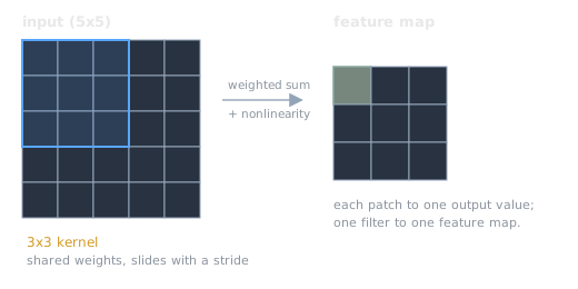
Convolution: local, shared weights
The core operation is convolution. A small filter (say 3x3 weights) is placed over a patch of the input, multiplied elementwise, and summed to one number, then a nonlinearity is applied. The filter then slides to the next patch and repeats. Two properties fall out:
- Local connectivity. Each output depends only on a small neighborhood, matching the fact that image structure is local.
- Weight sharing. The same filter weights are reused at every position, so the network learns a detector once and applies it everywhere. This is why a CNN has far fewer parameters than a fully connected net on the same image.
One filter produces one feature map, a grid showing where that feature appears. A layer learns many filters in parallel, so it outputs a stack of feature maps. Early layers tend to learn edges and color blobs; deeper layers combine those into textures, parts, and eventually objects, exactly the layered representation learning that defines deep learning in AI vs ML vs DL.
Stride, padding, receptive field
Sliding the filter one step at a time is stride one; larger strides skip positions and shrink the output. Padding the input border with zeros keeps the output from shrinking every layer. As you stack convolutions, each unit sees a larger patch of the original image, its receptive field, so depth is how a CNN goes from local edges to global structure.
How it learns
A CNN is trained like any other supervised network: a loss scores its predictions, and backpropagation with gradient descent adjusts the filter weights. The filters are not designed, they are learned from data, which is the whole break from the hand-engineered feature detectors that came before.
Why AlexNet mattered
The 2012 AlexNet result was a deep CNN that won ImageNet by more than ten percentage points over hand-engineered approaches. It learned better image features than decades of human feature engineering, and it ran because the matrix arithmetic of convolution maps perfectly onto GPUs. Downsampling and the deeper-network arc are covered in pooling and CNN architectures.
Related Notes
- Artificial Neural Networks, the fully connected baseline a CNN improves on
- Pooling and CNN Architectures, downsampling and the LeNet to ResNet arc
- Features and Representations, the layered features a CNN learns
- Backpropagation and Gradient Descent, how the filters are trained
- The Deep Learning Revolution, AlexNet and the GPU turning point
- AI vs ML vs DL, why learned features are the deep learning claim
Sources
- “Convolutional neural network,” Wikipedia. https://en.wikipedia.org/wiki/Convolutional_neural_network . Supports convolution with shared local filters, weight sharing, feature maps, stride/padding, receptive fields, and translation equivariance.
- Stanford CS231n, “Convolutional Networks.” https://cs231n.github.io/convolutional-networks/ . Supports local connectivity, parameter sharing, the layered edge-to-object feature hierarchy, and stride/padding mechanics.
- Goodfellow, Bengio, Courville, Deep Learning, MIT Press. https://www.deeplearningbook.org/contents/convnets.html . Supports convolution as the operation, sparse interactions, parameter sharing, and equivariant representations (Chapter 9).