A feedforward network eats a fixed-size input and is done. Text, audio, video, and biological sequences do not come in fixed sizes, and the meaning of step ten usually depends on steps one through nine. A recurrent neural network handles this with one structural trick: connections that point backward. The cell receives the current input plus its own output from the previous step, so it carries a running summary of everything it has seen.
The idea
A recurrent cell computes its output from the current input and its previous state, so the same small set of weights gets reused at every time step. Unrolled across a sequence, the RNN becomes a very deep network, and gradients flowing back through all those steps shrink toward zero (or blow up). Gated cells like the LSTM and GRU add an explicit memory that the network learns to write, keep, and erase, which is what makes long-range learning practical.
A cell with state
At time step t, a basic recurrent cell receives the input vector x(t) and its own previous output y(t-1). For a full layer with input weights Wx, recurrent weights Wy, bias b, and activation phi, the output is y(t) = phi(Wx^T x(t) + Wy^T y(t-1) + b). Because the output depends on the past, the cell effectively has memory: its hidden state h(t) = f(h(t-1), x(t)) acts as a learned summary of the input sequence so far, the sequence analogue of how convolutional layers summarize image features.
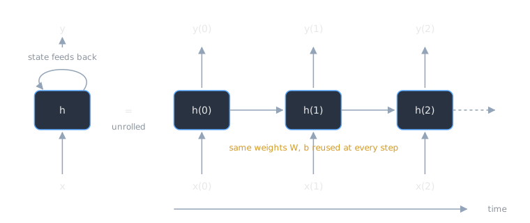
The same machinery supports several input-to-output shapes: sequence to sequence (predict the next value at every step), sequence to vector (read a whole review, emit one sentiment score), vector to sequence (one image in, a caption out), and the encoder-decoder combination that powered early neural machine translation, where an encoder RNN compresses the input sentence into a context vector and a decoder RNN expands it into the target language.
Training by unrolling
Training treats the unrolled network as one deep computation graph, a technique called backpropagation through time (BPTT). Forward-pass a sequence, score the output sequence with a loss such as a weighted sum of cross-entropies, then run backpropagation backward through the unrolled graph, summing each weight’s gradient contributions across all time steps before the gradient-descent update. The catch is that every time step adds depth, so a 100-step sequence behaves like a 100-layer network with tied weights.
The vanishing gradient problem
Gradients flowing backward through long paths get multiplied by roughly the same factors at every step. If those factors are smaller than one the gradient shrinks exponentially and early time steps learn almost nothing; if larger than one it explodes. The problem was identified in Sepp Hochreiter’s 1991 diploma thesis, and it is the reason plain RNNs struggle to connect a word to context from fifty words earlier. Exploding gradients have a blunt but effective fix, clipping the gradient to a bounded range. Vanishing gradients needed an architectural fix.
LSTM: learning what to remember
The Long Short-Term Memory cell, introduced by Hochreiter and Schmidhuber in 1997, splits the state in two: a short-term state h(t) and a long-term cell state c(t). Three learned gates, each a sigmoid layer reading x(t) and h(t-1), control the flow. The forget gate (a later refinement, added around 2000) decides what to erase from c(t-1), the input gate decides what new information to write, and the output gate decides what part of the long-term state becomes the output h(t). Because the cell state is updated additively rather than being squashed through an activation at every step, gradients can flow across long spans without dying, and the network learns from data what is worth remembering.
GRU: the simplified gate
The Gated Recurrent Unit came out of Cho et al.’s 2014 work on RNN encoder-decoders for machine translation. It merges the LSTM’s cell state and hidden state into one vector and collapses the forget and input gates into a single update gate z(t): whatever fraction of the old state is kept, one minus that fraction of the new candidate is added. A reset gate r(t) controls how much of the previous state feeds the candidate. Fewer parameters, similar performance in many settings, same core trick of gated additive memory.
Sequence to vector in practice
Sentiment analysis of a movie review is the classic sequence-to-vector setup: feed the review through the RNN one token at a time (each token converted to a vector by an embedding layer), ignore the intermediate outputs, and read the final state as a summary of the whole review, which a last layer maps to a sentiment score.
Recurrence had a strong run in NLP, then attention mechanisms and the transformer architecture (attention without recurrence) took over the state of the art, partly because transformers train faster and suffer less from vanishing gradients. The gated-memory idea still matters: it is the cleanest illustration of how an architectural change, not more data, solved a fundamental optimization failure in the deep learning era.
Related Notes
- Artificial Neural Networks, the feedforward foundation the recurrent cell extends
- Backpropagation, the algorithm BPTT unrolls across time
- Gradient Descent, the update rule the summed gradients feed
- Loss Functions, how an output sequence gets scored
- Embeddings, the learned word vectors an RNN consumes as input
- Features and Representations, the state vector as a learned summary
- The Deep Learning Revolution, the era these architectures defined
- AI vs ML vs DL, where sequence models sit in the bigger picture
Sources
- Goodfellow, Bengio, Courville, Deep Learning, Chapter 10: Sequence Modeling: Recurrent and Recursive Nets. https://www.deeplearningbook.org/contents/rnn.html . Supports the recurrent computation with shared parameters across time steps, backpropagation through time on the unrolled graph, the long-term dependency (vanishing/exploding gradient) challenge, and gated architectures (LSTM, GRU) as the response.
- “Recurrent neural network,” Wikipedia. https://en.wikipedia.org/wiki/Recurrent_neural_network . Supports RNNs processing variable-length sequences via hidden state, the unrolling view, and the encoder-decoder application to machine translation.
- “Vanishing gradient problem,” Wikipedia. https://en.wikipedia.org/wiki/Vanishing_gradient_problem . Supports the identification of the problem in Hochreiter’s 1991 diploma thesis, exponential shrinking of backpropagated gradients over long paths, and gradient clipping as a mitigation for explosions.
- “Long short-term memory,” Wikipedia. https://en.wikipedia.org/wiki/Long_short-term_memory . Supports the LSTM’s introduction by Hochreiter and Schmidhuber in 1997, the input/output gate structure with the forget gate added circa 2000, the cell-state and hidden-state split, and the gates’ role in preserving gradient flow.
- Cho et al., “Learning Phrase Representations using RNN Encoder-Decoder for Statistical Machine Translation” (2014). https://arxiv.org/abs/1406.1078 . Supports the 2014 origin of the gated hidden unit that became the GRU, inside an RNN encoder-decoder for machine translation.
- “Gated recurrent unit,” Wikipedia. https://en.wikipedia.org/wiki/Gated_recurrent_unit . Supports the GRU’s 2014 introduction by Kyunghyun Cho and colleagues, its update/reset gate structure, and its having fewer parameters than the LSTM.