Breadth-First Search

Overview

Breadth-First Search (BFS) explores a graph in layers: it visits all vertices at distance k from a source before moving to distance k+1.
Implemented with a queue, BFS provides:

• Reachability (which vertices are connected to the source),
• Shortest-path distances in unweighted graphs (edge cost = 1),
• A parent tree (or BFS tree) suitable for reconstructing paths.

Note

BFS discovers vertices in nondecreasing distance from the source. The first time a vertex is dequeued is the moment we know its final shortest distance (in edges) from the source.

---

Model & Invariants

Let G = (V, E) be a directed or undirected graph. Choose a source s ∈ V.

State tracked by BFS:

• dist[v] — distance in edges from s to v (∞ if unreached),
• parent[v] — predecessor of v on a shortest path from s,
• visited[v] — whether v has been discovered (enqueued).

Invariants maintained during the algorithm:

1. The queue contains vertices in nondecreasing dist.
2. When we dequeue a vertex u, all vertices at distance < dist[u] have already been fully processed.
3. An edge (u, v) that first discovers v sets
   dist[v] = dist[u] + 1 and parent[v] = u.

Tip

Mark vertices visited at enqueue time (not at dequeue). This prevents multiple enqueues of the same vertex.

---

Pseudocode (Adjacency List)

function BFS(Adj, s):
    for v in V:
        dist[v] = ∞
        parent[v] = NIL
        visited[v] = false
    dist[s] = 0
    visited[s] = true
    Q = empty queue
    enqueue(Q, s)
 
    while not empty(Q):
        u = dequeue(Q)
        for v in Adj[u]:
            if not visited[v]:
                visited[v] = true
                dist[v] = dist[u] + 1
                parent[v] = u
                enqueue(Q, v)

• Adj[u] yields neighbors of u.

• On undirected graphs, edges are stored symmetrically; on directed graphs, only out-neighbors appear.

---

Correctness Sketch (Shortest Paths)

Claim: After BFS completes, for any vertex v reachable from s, dist[v] equals the length of a shortest path (number of edges) from s to v.

Idea:

• BFS examines vertices in increasing distance from s.

• The first time v is discovered, it must be via an edge (u, v) from some u already at minimum distance; thus dist[v] = dist[u] + 1 is minimal.

• By induction on distance layers, no smaller distance can exist.

---

Reconstructing Paths (Parent Tree)

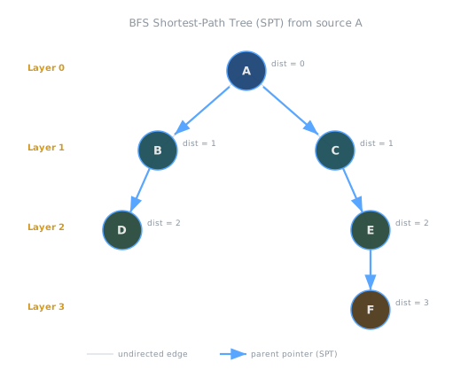
BFS implicitly builds a shortest-path tree (SPT) rooted at s.

function reconstructPath(parent, s, t):
    if parent[t] == NIL and t != s:
        return []   // unreachable
    path = []
    cur = t
    while cur != NIL:
        push_front(path, cur)
        cur = parent[cur]
    return path

• The returned path lists vertices from s to t.

• For all reachable t, this path length equals dist[t].

---

Complexity & Data Structures

Assume adjacency lists with n = |V|, m = |E|.

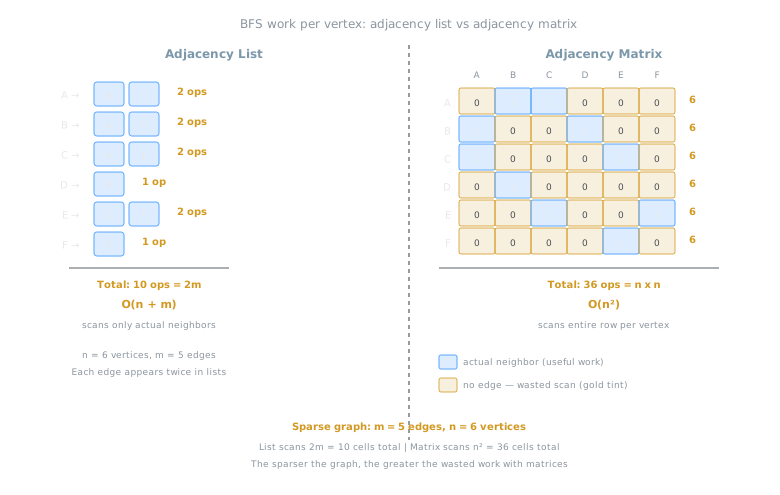
• Time: Θ(n + m) — each vertex enqueued once; each edge examined at most twice (undirected) or once (directed).

• Space: Θ(n) for dist, parent, visited, plus the queue.

With an adjacency matrix, scanning neighbors costs Θ(n) per vertex, so total time is Θ(n²).

Tip

Prefer adjacency lists for sparse graphs (m ≪ n²); matrices can be reasonable for dense graphs or when hasEdge(u, v) queries are frequent.

---

Multi-Source BFS

To compute distance from a set of sources S (e.g., nearest facility):

function multiSourceBFS(Adj, S):
    for v in V:
        dist[v] = ∞; parent[v] = NIL; visited[v] = false
    Q = empty queue
    for s in S:
        dist[s] = 0
        visited[s] = true
        enqueue(Q, s)
    while not empty(Q):
        u = dequeue(Q)
        for v in Adj[u]:
            if not visited[v]:
                visited[v] = true
                dist[v] = dist[u] + 1
                parent[v] = u
                enqueue(Q, v)

This effectively treats S as a super-source with zero edges to all s ∈ S.

---

Disconnected Graphs & All-Pairs Coverage

To visit all components, run BFS from each unvisited vertex:

for each v in V:
    if not visited[v]:
        BFS(Adj, v)

• This produces a BFS forest (one BFS tree per component).

• For all-pairs shortest paths in unweighted graphs, run BFS from each source (or use specialized methods if needed).

---

Directed vs Undirected, Weighted vs Unweighted

• Undirected graphs: BFS layers alternate by distance, edges always connect the same or adjacent layers (k ↔ k+1).

• Directed graphs: Outgoing edges determine reachability; distances respect direction.

• Weighted graphs: BFS computes shortest paths only when all edges have equal weight (or unit weight).
  For nonnegative weights, use Dijkstra’s algorithm; for negative edges without cycles, use Bellman–Ford.

Warning

Do not use BFS for general weighted graphs; results are not shortest paths unless all weights are identical.

---

Common Pitfalls

Warning

Visited at the wrong time:
Marking visited[v] after dequeue may enqueue v multiple times, inflating complexity and breaking invariants. Mark at enqueue.

Warning

Forgetting to initialize dist to ∞:
Uninitialized distances can be mistaken for zero and corrupt path lengths.

Warning

Mishandling directed graphs:
Ensure adjacency lists reflect outgoing edges; undirected graphs require symmetric storage.

Tip

To save memory when you only need reachability, you can omit dist and parent and keep a boolean visited plus the queue.

---

Worked Example

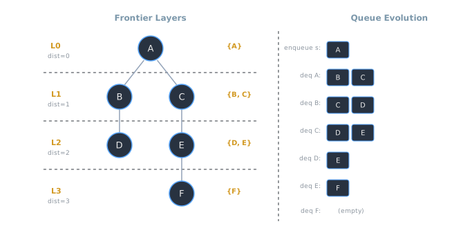
Consider G (undirected), V = {A, B, C, D, E, F}, edges:
A—B, A—C, B—D, C—E, E—F.

BFS from A:

1. Init: dist[A]=0, enqueue A.

2. Dequeue A → discover B, C (set dist=1, parent=A), enqueue both.

3. Dequeue B → discover D (set dist=2, parent=B).

4. Dequeue C → discover E (set dist=2, parent=C).

5. Dequeue D → no new neighbors.

6. Dequeue E → discover F (set dist=3, parent=E).

7. Dequeue F → done.

Shortest path A → F reconstructed by chasing parents: F ← E ← C ← A (reverse to get forward order).

---

Applications

• Shortest paths in unweighted graphs (routing on hop count).

• Level decomposition (topological layers in DAG-like BFS on unweighted edges).

• Bipartite testing (2-coloring via levels: even/odd parity).

• Finding connected components (with multiple BFS runs or union-find).

• Web crawling and network flood-fill approximations.

Tip

Bipartite check: Color source as 0; neighbors as 1; next layer as 0; if any edge connects same colors, the graph is not bipartite.

---

Implementation Notes

• Queue choice: language-provided double-ended queues (deque) offer O(1) amortized enqueue/dequeue.

• Memory footprint: store parent as int16/int32 when vertex IDs fit; distances can use int32 or int64.

• Edge iteration: favor contiguous adjacency vectors for cache locality.

---

Summary

• BFS is a layered, queue-based traversal that guarantees shortest-path distances in unweighted graphs.

• It runs in Θ(n + m) with adjacency lists.

• The parent tree enables path reconstruction.

• Use multi-source BFS for nearest-source problems and repeat BFS to cover disconnected components.

---

See also

• Depth-First Search (DFS)

• Graph Representations

• Dijkstra’s Algorithm

• Adjacency List

• Adjacency Matrix