Splay Tree

Overview

A splay tree is a binary search tree (BST) that self-adjusts by performing a splay operation after every access (search, insert, delete). Splaying repeatedly rotates the accessed node x toward the root using one of three local patterns—zig, zig–zig, or zig–zag—until x becomes the root. While a single operation can take linear time in the worst case, any sequence of m operations on a tree with n keys costs amortized O(log n) per operation. Splay trees adapt to temporal locality and offer powerful “static/working-set” performance properties without storing balance information.

Note

Splay trees maintain the standard BST invariant: for every node u, all keys in u.left are < u.key and all keys in u.right are > u.key.

Structure Definition

Each node stores key, optional value, and pointers to left, right, and (optionally) parent:

struct Node {
  key: K
  value: V
  left: Node*
  right: Node*
  parent: Node*  // optional, but simplifies rotations
}

No explicit balance factors or colors are kept—shape is implicit and continuously adjusted by splaying.

• Root: last accessed node after every public operation.

• Empty tree: root = NIL.

• Duplicates: typically disallowed or handled by a side policy (e.g., count field).

Core Operations

All public operations end by splaying the last touched node (or the parent of a removed node) to the root.

Splay primitive

Splaying rotates x up until it becomes root using:

• Zig: x is a child of the root → single rotation.

• Zig–zig: x and its parent p are both left children or both right children → rotate p then x (two rotations in the same direction).

• Zig–zag: x is a left child and p is a right child, or vice versa → rotate x over p, then rotate x over g (the grandparent).

function SPLAY(root, x):
    while x.parent ≠ NIL:
        p = x.parent
        g = p.parent
        if g == NIL:                       // Zig
            ROTATE(root, x)
        else if (x == p.left and p == g.left) or (x == p.right and p == g.right):  // Zig–zig
            ROTATE(root, p)
            ROTATE(root, x)
        else:                              // Zig–zag
            ROTATE(root, x)
            ROTATE(root, x)
    return x  // new root

ROTATE(root, x) is the standard single BST rotation that raises x above its parent, updating parent/child pointers (and the root if needed).

Search

function SEARCH(root, key):
    cur = root; last = NIL
    while cur ≠ NIL and cur.key ≠ key:
        last = cur
        if key < cur.key: cur = cur.left else: cur = cur.right
    if cur == NIL:
        // splay the last accessed node to root (predecessor/successor candidate)
        if last ≠ NIL: root = SPLAY(root, last)
        return (root, NIL)
    else:
        root = SPLAY(root, cur)
        return (root, cur)

Insert

Standard BST insert, then splay the new node.

function INSERT(root, key, value):
    if root == NIL: return new Node(key,value)
    cur = root; parent = NIL
    while cur ≠ NIL:
        parent = cur
        if key < cur.key: cur = cur.left
        else if key > cur.key: cur = cur.right
        else: cur.value = value; return SPLAY(root, cur)  // update existing
    x = new Node(key,value, NIL,NIL,parent)
    if key < parent.key: parent.left = x else: parent.right = x
    return SPLAY(root, x)

Delete

Splay the target (or last accessed) to root; then splice subtrees.

function DELETE(root, key):
    (root, x) = SEARCH(root, key)
    if x == NIL: return root
    // x is root now
    L = x.left;  R = x.right
    if L ≠ NIL: L.parent = NIL
    if R ≠ NIL: R.parent = NIL
    free(x)
    if L == NIL: return R
    // bring the maximum of L to root so we can attach R as its right child
    // find rightmost in L
    y = L
    while y.right ≠ NIL: y = y.right
    L = SPLAY(L, y)     // y becomes root of L; it has no right child
    L.right = R
    if R ≠ NIL: R.parent = L
    return L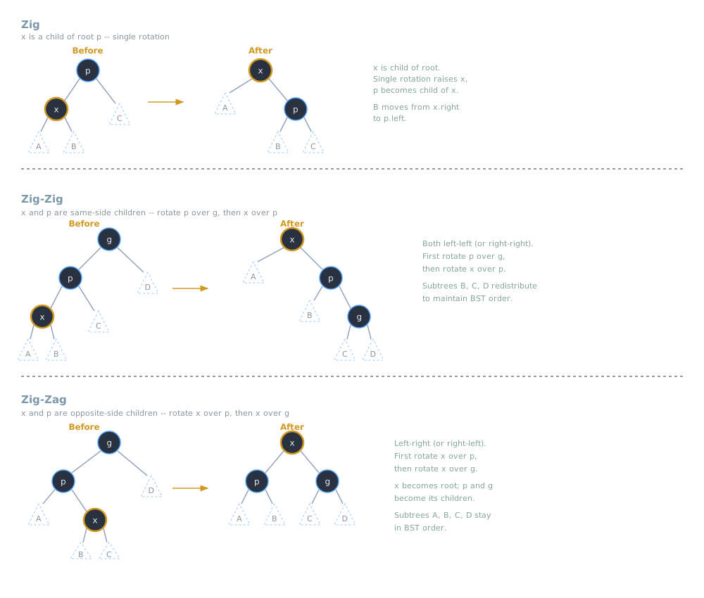

Example (Stepwise)

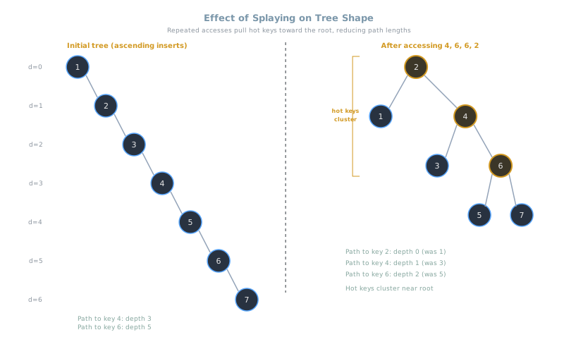
Consider starting with a skewed BST on keys [1,2,3,4,5,6,7] (ascending inserts). Access sequence: 4, 6, 6, 2.

1. Access 4: found under the right spine; splaying 4 applies zig–zig rotations and makes 4 the root. Subtrees [1..3] and [5..7] hang as left/right.

2. Access 6: go right from 4 (5 then 6); perform a zig–zig (if 6 is right child of right child) to bring 6 to root. Hot key rises quickly.

3. Access 6 again: 6 is already root → zig not needed; cost is O(1).

4. Access 2: descend into left subtree and splay 2 to the root via zig–zag / zig–zig as needed.

Note

Repeatedly accessed elements migrate near the root, yielding fast subsequent hits. This demonstrates the working-set behavior even without explicit metadata.

Complexity and Performance

• Worst-case per operation: O(n) (a long path can be rotated up).

• Amortized over a sequence: O(log n) per operation. The standard potential-function proof shows total time across m operations is O(m log n + n log n).

• Sequential access property: Scanning keys in sorted order takes amortized O(1) per access after the first few steps due to tree reconfiguration.

• Static optimality (informal): Over long runs, splay trees compete (within a constant factor) with the best fixed BST for the observed access distribution.

• Working-set bound (informal): Access cost to an element is O(log t) where t is the number of distinct items accessed since its last access.

Tip

In practice, splay trees shine when temporal locality is strong: recently accessed keys remain near the top, minimizing future access time.

Implementation Details or Trade-offs

• Parent pointers vs recursion: Parent pointers simplify SPLAY and ROTATE. A parent-less implementation is possible with explicit stacks but is more complex.

• Top-down splaying: An alternative “split-while-descend” style avoids parent pointers, maintaining two temporary trees (leftTree, rightTree) and reassembling around the accessed key. This can reduce pointer chasing.

• Join/Split primitives:

  • SPLIT(root, key) → (L, R) such that all keys in L < key and all keys in R ≥ key (splay at key or predecessor).

  • JOIN(L, R) requires max(L) < min(R): splay max(L) to make it root with empty right child, then attach R as root.right.

• Memory locality: Like other pointer-rich trees, splay trees can suffer cache misses. Top-down variants can have better locality due to fewer parent-pointer dereferences.

• No balance metadata: Simpler node structure than AVL Tree or Red–Black Tree, at the cost of per-operation variance.

Practical Use Cases

• Caches and dictionaries with skewed access distributions (Zipf-like), where recency dominates.

• Move-to-root heuristics for symbol tables and compiler passes where the working set shifts as you traverse code.

• Join/Split-based sets and maps, where splitting around a pivot and joining later is common (e.g., range updates).

• Memory-constrained settings that benefit from simple nodes (no color/balance fields) and amortized guarantees.

Tip

If you often need order statistics (k-th element, rank), consider augmenting nodes with subtree sizes. Rotations must update sizes on the fly.

Limitations / Pitfalls

Warning

Unpredictable latency. Individual operations can take Θ(n) time. If you need hard worst-case bounds per operation, prefer Red–Black Tree or AVL Tree.

Warning

Deletion nuances. After splaying the target to root, you must carefully JOIN left and right subtrees (often by splaying the max of the left subtree). Errors here easily violate the BST invariant.

Warning

Sequential patterns. While splay trees have good properties for scans, some workloads interleaving long runs with sparse accesses can temporarily degrade shape; consider top-down splaying and batching joins/splits.

Warning

Concurrency. Fine-grained locking is tricky because splaying changes paths all the way to the root. For high-concurrency maps, lock-free skip lists or balanced trees with localized rotations may be easier.

Summary

Splay trees are metadata-free, self-adjusting BSTs: every access performs splaying to move the touched node to the root using zig, zig–zig, and zig–zag rotations. They guarantee amortized O(log n) cost per operation over sequences, adapt naturally to temporal locality, and provide elegant split/join operations. The trade-off is unbounded per-operation latency and sensitivity to rotation correctness during deletion and bulk updates. When workloads feature hot keys and shifting working sets, splay trees offer a compact, practical alternative to strictly balanced trees.

See also

• Binary Search Tree

• AVL Tree

• rb-tree

• Trees