Types of Binary Tree

Overview

Binary trees come in many flavors—full (proper), complete, perfect, and balanced—each imposing structural constraints that affect height, memory layout, and operation costs. Understanding these definitions and how they interact prevents ambiguous claims (“this tree is balanced”) and helps choose or prove properties of data structures like heaps, BSTs, and search indexes.

Note

A binary tree restricts each node to at most two children: left and right. See Binary Tree for fundamentals and Tree Traversal — Overview for visiting orders.

Motivation

• Performance guarantees: Balanced forms bound height to Θ(log n), yielding logarithmic search/update in BST-like structures.
• Memory/layout: Complete trees admit array layouts with simple index formulas (heaps).
• Reasoning & proofs: Clear terminology avoids mixing incompatible properties (e.g., “full” vs “complete”).

Definition and Formalism

Let n be the number of nodes and h the height (length in edges on the longest root-to-leaf path), with the convention height(leaf)=0 and height(empty)=-1.

• Full (proper) binary tree: Every internal node has exactly two children. Leaves may appear at different depths.
  • Example shapes:

        •            •
       / \          / \
      •   •        •   •
                 / \
                •   •
    

• Complete binary tree: All levels are completely filled except possibly the last, which is filled from left to right without gaps.
  • Precisely the shape used by heaps (array index formulas apply).
• Perfect binary tree: All internal nodes have two children and all leaves are at the same depth.
  • Exact counts: n = 2^{h+1} − 1 and leaves L = 2^h.
• Balanced (height-bounded) binary tree: Informally, one whose height is Θ(log n). Formalisms vary by scheme:
  • AVL: for every node, |height(left) − height(right)| ≤ 1.
  • Red–black: a BST with a coloring invariant; every root-to-leaf path has the same black-height. Guarantees h ≤ 2 ⌊log2(n+1)⌋.
  • Weight-balanced (e.g., scapegoat trees): subtree sizes are bounded by ratios.
  • Treaps/splay: achieve expected or amortized logarithmic height/operations (probabilistic/self-adjusting balance).

Warning

“Balanced” is not a single canonical property. Always state which balancing scheme or height bound you mean.

Shape Comparison

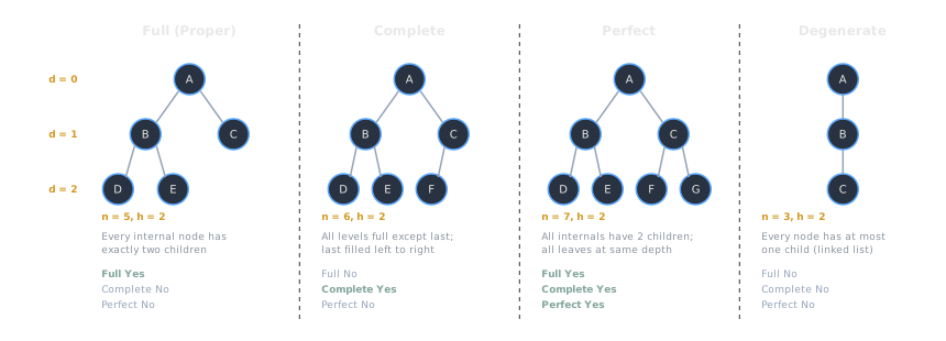
Each panel shows a minimal witness tree with its Full / Complete / Perfect classification. Note that Perfect ⇒ Full ∧ Complete, but neither Full nor Complete alone implies the other.

Properties and Relationships

• Implications:
  • Perfect ⇒ Full and Complete.
  • Complete ⇏ Full (last level can be partially filled).
  • Full ⇏ Complete (levels can be uneven).
  • Any of {Full, Complete, Perfect} do not alone imply “balanced,” though Perfect has h = ⌊log2(n)⌋ and Complete has h = ⌊log2(n)⌋ or ⌊log2(n)⌋ + 1.
• Height bounds:
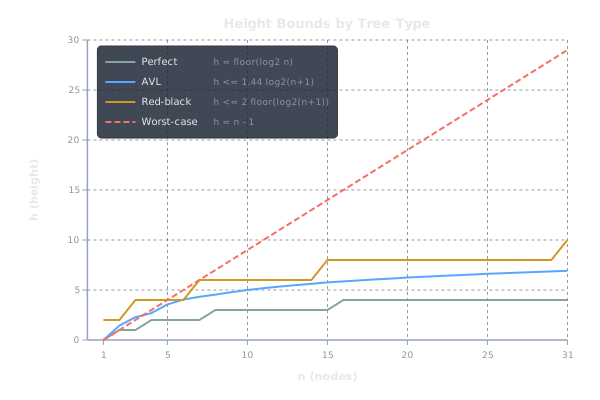
  • Perfect: h = ⌊log2(n)⌋.
  • Complete: h = ⌊log2(n)⌋ or ⌊log2(n)⌋ + 1.
  • AVL: h ≤ c · log2(n+1) with c ≈ 1.44 (tight bound using Fibonacci-like recurrences).
  • Red–black: h ≤ 2 · ⌊log2(n+1)⌋.
  • Degenerate (path): h = n − 1.
• Leaf/internal counts (full trees): In a full binary tree, #leaves = #internal + 1.
  Proof sketch: Sum of out-degrees is n − 1; full internal nodes each contribute 2, so 2I = n − 1 with n = I + L ⇒ L = I + 1.
• Array layout (complete trees): With 0-based indexing, parent/child indices satisfy:
  • left(i) = 2i + 1, right(i) = 2i + 2, parent(i) = ⌊(i − 1)/2⌋.
    This requires completeness to avoid holes; see Binary Heap.

Tip

When proving logarithmic time for heap or BST variants, reduce to a height bound using the tree’s structural/ balance invariant, then show the algorithm’s path length is O(h).

Implementation or Practical Context

• Heaps (priority queues): Require complete binary shape; do not need “full” or “perfect.” Array representation minimizes pointers and improves cache locality. See Heaps — Overview and Heapify.
• Balanced BSTs (maps/sets): Need height-bounded trees. Choices:
  • AVL: tighter height ⇒ faster lookups; more rotations on updates.
  • Red–black: looser bound but fewer rotations; common in libraries.
  • Splay: no explicit height invariant; amortized logarithmic access; good locality for skewed access patterns. See AVL Tree, Red–Black Tree, Splay Tree.
• Memory/layout trade-offs:
  • Pointer-based nodes are flexible but may be cache-inefficient on large trees.
  • Array-based layouts exploit completeness; random access and sequential scans are fast.
• Static vs dynamic: For static, read-mostly data, building a perfect or nearly complete shape can maximize cache performance and allow binary-search-like traversals over arrays.

Common Misunderstandings

Warning

“Full = all levels filled.” No—full means every internal node has two children; levels can still be ragged. “All levels filled” is part of complete or perfect definitions.

Warning

“Complete implies perfect.” False. A complete tree’s last level may not be full; perfect requires all leaves at the same depth.

Warning

“Balanced means AVL.” “Balanced” is ambiguous. It might mean AVL balance (|Δheight| ≤ 1), red–black constraints, weight balance, or simply h = Θ(log n). State the scheme.

Warning

Using heap index formulas on non-complete trees. Sparse shapes break 2i+1/2i+2 relations and waste memory.

Warning

Depth vs height off-by-one. Adopt consistent conventions: height(leaf)=0, height(empty)=-1, depth(root)=0. See Trees — Overview.

Example: Height Bounds by Type

Consider the following node counts and the implied heights:

• n = 1 ⇒ perfect & complete ⇒ h = 0.
• n = 10:
  • Perfect lower bound: h ≥ ⌈log2(10+1)⌉ − 1 = 3.
  • Complete: h is 3 or 4 depending on last-level fill.
  • AVL: h ≤ ⌊1.44 · log2(11)⌋ = 4 (tight-ish).
  • Red–black: h ≤ 2 · ⌊log2(11)⌋ = 6.
• n = 2^{h+1} − 1 ⇒ perfect with height h; any missing leaf at the last level makes it complete but not perfect.

Balanced Families (At a Glance)

• AVL Trees: Strict local balance via height differences. Guarantees h ≤ 1.44 log2(n+2) − 1.328 (classical bound). Excellent lookup times; rotations on updates may be more frequent.
• Red–Black Trees: Color invariant ensures paths differ in length by at most a factor of 2. Ubiquitous in standard libraries due to good update performance and simpler invariants.
• Splay Trees: No static bound on height, but amortized O(log n) access; excels on temporal locality and access sequences.
• Weight-/Size-balanced: Keep subtree sizes within fixed ratios; provide deterministic O(log n) with simpler implementations in some cases.

Tip

If you need stable worst-case O(log n) and minimal update overhead, red–black is often a pragmatic default. If you need near-optimal lookup height (read-heavy), AVL can shine.

Broader Implications

• Asymptotics from structure: Bounding h = Θ(log n) generally implies logarithmic-time search/insert/delete along root-to-leaf paths in BST-like trees.
• Cache and SIMD: Nearly complete or perfect layouts are friendlier to prefetching and can accelerate range queries with contiguous memory.
• Parallelism: Subtree independence enables parallel traversals; perfect/complete trees simplify work partitioning by levels.

Summary

Binary-tree “types” encode shape constraints:

• Full (proper): every internal node has two children.
• Complete: all levels full except possibly the last, filled left to right (heap-friendly).
• Perfect: both full and leaves at the same depth (tightest h = ⌊log2(n)⌋).
• Balanced: umbrella for height-bounded schemes (AVL, red–black, etc.), aiming for h = Θ(log n).

Know which property you need: complete for heaps and array layouts, balanced for logarithmic operations in BSTs, perfect mainly as a theoretical ideal. Use precise definitions to avoid ambiguity and to translate structure into performance guarantees.

See also

• Binary Tree
• Heaps — Overview
• AVL Tree
• rb-tree